© 2008 Rasmus ehf and Jóhann Ísak
|
© 2008 Rasmus ehf and Jóhann Ísak |
Vectors |
|
Parametric equations and polar coordinates
We have seen how to find the coordinates of a point by using position vectors and vector addition. (See lesson 3). If we knew the direction of the vector we could control the length by multiplying by a number that we called t.
We can find a vector equation of a line if we know a fixed point that the line
goes through, P1 = (x1,y1)
and a direction vector
![]() for the line..
for the line..
If P is any point on the line, we can write the position vector for P
![]() =
= ![]() + t·
+ t·![]()
or using coordinates:
![]()
This form of the equation of a straight line is called the parametric form, t is called a parameter. We usually write this vector equation as two linear equations, one for the x coordinate and the other for the y coordinate.
|
If (x1, y1)
is a point on the line
and
|
The parameter t takes different values for different points on the line and is therefore the variable in the equation.
Find the parametric equation of the line y = 3x + 2.
The general form of the equation is 3x – y + 2 = 0 so the normal vector of the
line is
![]() and the direction vector is
and the direction vector is ![]()
We find any point on the line by choosing, for example, x = 1 and calculating y = 3·1 + 2 = 5 . This tells us that (1, 5) is a point on the line. The parametric form of the equation is therefore:
|
|
x = 1 + t y = 5 + 3t |
By choosing different values of t we can find the coordinates of points on the line.
For example if t = 1 then we get x = 1 + 1 = 2 and y = 5 + 3·1 = 8, giving us the point (2, 8) on the line.
Choosing t = 2 we get x = 1 + 2 = 3 and y = 5 + 3·2 = 11 telling us that (3, 11) is on the line.
If we want to find y when x = 4 we find the value of t that corresponds to x = 4 and use that to find y.
x = 1 + t = 4
t = 4 – 1 = 3
y = 5 + 3·3 = 14
Change the parametric equation in example 1 back to its original form. We do this by eliminating t.
|
|
x = 1 + t gives t = x – 1 y = 5 + 3t gives t = (y – 5)/3 |
The t is the same value in both equations so we can write an equation.
x – 1 = (y – 5)/3
3x – 3 = y – 5
3x + 2 = y
Which is the same equation as in example 1.
Is the point (100, 302) on the line with parametric equation
|
|
x = 1 + t y = 5 + 3t |
We use the coordinates given to find t from both equations.
|
|
100 = 1 + t gives t = 99 302 = 5 + 3t gives t = (302 – 5)/3 = 297/3 = 99 |
We get the same value for t from both equations telling us that the point (100, 302) lies on the line.
Find the point of intersection of the two lines that have the parametric equations:
|
|
x = 1 + 2t y = 1 + t |
and
|
|
x = 6 + 3r y = 1 – r |
We use different labels for the parameters t and r because these are two different equations with different variables. In the point where the lines intersect, the x and y values must be the same in both equations. This gives us simultaneous equations that can be solved.
x = 1 + 2t = 6 + 3r
and
y = 1 + t = 1 – r
giving the equations
|
|
2t – 3r = 5 t = –r |
Inserting –r into the first equation instead of t gives us
2(–r) – 3r = 5
–5r = 5
r = –1 and therefore t = 1
This means we can find x and y by putting either t or r into the equations for x and y. Using the value for t gives us
|
|
x = 1 + 2t = 1 + 2·1 = 3 y = 1 + t = 1 + 1 = 2 |
Check by putting the r value in.
|
|
x = 6 + 3r = 6 + 3(–1) = 3 y = 1 – r = 1 – (–1) = 2 |
The point of intersection is (3, 2).
The parametric form of an equation is extremely useful, not only for finding the equation of a straight line. In many cases, we can easily find the parametric equation although we can‘t find an ordinary x – y equation. The parametric form involves finding separate equations for x and y using the parameter t. By choosing values of t we find the values of x and y that correspond to that t value.
If we call the functions f and g respectively we can write:
|
|
x = f(t) y = g(t) |
Finding an x, y equation involves eliminating t from these two equations as we saw in the above examples.
Change the following parametric equation into an x –y equation:
|
|
x = t + 1 y = t2 – 1 |
From the first equation we get t = x – 1 and therefore t2 = x2 – 2x + 1
From the second equation we get t2 = y + 1. Equating these two expressions for t2 we get:
y + 1 = x2 – 2x + 1
y = x2 – 2x
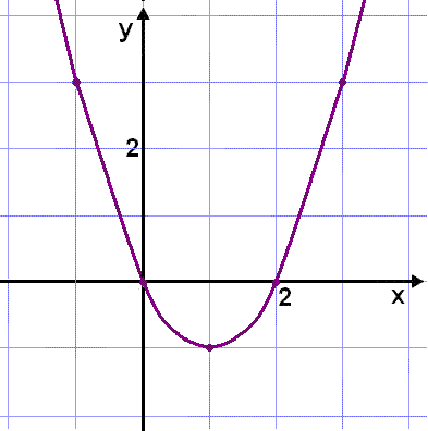
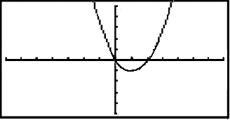
This is the equation of a parabola that crosses the x axis in the points where x = 0 and x = 2. ( found by solving for x when y = 0)
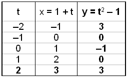
We can draw the graph of a function given in parametric form by choosing values of t and finding both x and y . We have chosen t values from –2 to 2.
 |
 |
|
We can see that it is just as |

We can use the CASIO graphical calculator to draw graphs given in parametric
form in the same way as we can use it to draw graphs given in the x- y form.
First choose GRAPH and then the V-Window using
We get the following menu:
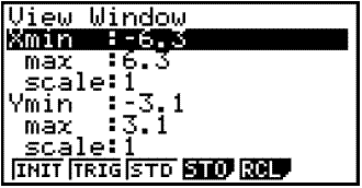
By pushing the down arrow five times we reach the bottom of this menu. If we push the down arrow once more a new menu window appears.
 |
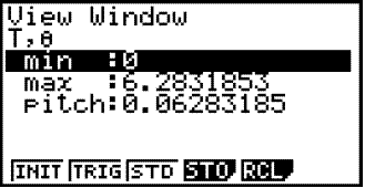 |
We now choose t values,
![]() doesn‘t matter for the moment. We will choose the same values as we used in the
table above, from -2 to 2. If we use pitch 1 the graph will look as if it is
made up of short line segments. The smaller we choose the pitch, the smoother
the graph.
doesn‘t matter for the moment. We will choose the same values as we used in the
table above, from -2 to 2. If we use pitch 1 the graph will look as if it is
made up of short line segments. The smaller we choose the pitch, the smoother
the graph.
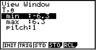
Finally we use the
![]() button
button
This will take us back to the graph window.
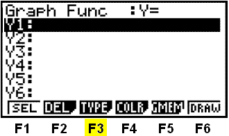
We choose a new type of graph with (TYPE) using F3. A new menu window comes up:
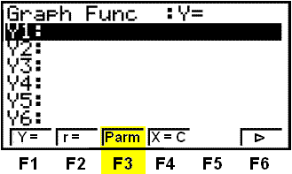
We are using the parametric form so we choose (Parm) by pressing F3. The graph window comes up again this time allowing us to write in equations for both x and y (shaded).
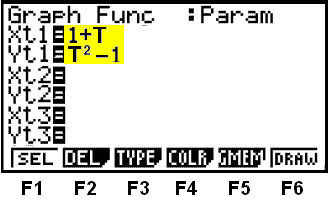
The T in the formula is on the same button on the calculator as the x that we
have previously used
![]()
This is what the graph looks like:
Look at the following parametric equation:
|
|
x = 4 + 2 cos t y = 3 + 2 sin t |
We solve these equations for t by squaring both equations, adding together and then using the rule cos2 t + sin2 t = 1 to eliminate t.
Rearranging the x equation gives x – 4 = 2 cos t and then squaring, we get (x – 4)2 = 4 cos2t.
Working with the y equation in the same way, we get y – 3 = 2 sin t and (y – 3)2 = 4 sin2t.
Adding the two equations together gives us:
(x – 4)2 + (y – 3)2 = 4 cos2 t + 4 sin2 t
= 4(cos2 t + sin2 t)
= 4
The result is the equation (x – 4)2 + (y – 3)2 = 22 which is the equation of a circle with radius 2 and centre in (4, 3).
In the above lesson a new method, the parametric method, for writing equations has been introduced. x and y are calculated separately using the variable, or parameter, t.
There are many different coordinate systems that can be used, the x and y axis do not need to be perpendicular or have the same units of scale.
We are now going to study another type of coordinates called polar coordinates. The system has only one axis, corresponding to the positive part of the old horizontal x axis. We call it the polar axis or the initial ray. The origin of the system is often called the pole.
All points in the plane can be found by giving their distance, r, from the
origin and the angle
![]() that they make with the polar axis (see the diagram). The polar coordinates of a
point are (r,
that they make with the polar axis (see the diagram). The polar coordinates of a
point are (r,
![]() ).
).
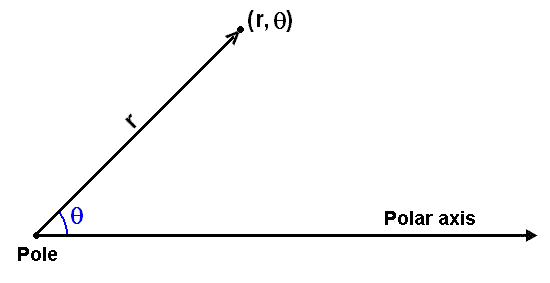
The distance r is directed, like a vector, and therefore can be negative. If the
angle
![]() is on the interval 0
<
is on the interval 0
<
![]() <
<
![]() (0º
<
(0º
<
![]() <
180º), a negative value of r means that the point lies below the polar axis. The
angle
<
180º), a negative value of r means that the point lies below the polar axis. The
angle
![]() is measured anti clockwise from the pole axis. It can also be negative.
is measured anti clockwise from the pole axis. It can also be negative.
We can place a point in the x-y coordinate system using polar coordinates if we let the polar axis correspond to the x axis and the pole be in the point (0, 0).
Find the polar coordinates of the point (3, 4).
We begin with a diagram.
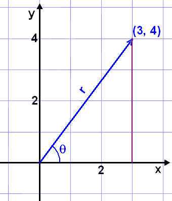
We see straight away that we can use Pythagoras Rule to find r.
r2 = 32 + 42 = 9 + 16 = 25
r = 5
We need to use the rules of trigonometry in a right angled triangle to find ![]() .
tan
.
tan
![]() = opposite side/adjacent side which gives us:
= opposite side/adjacent side which gives us:
![]() = tan–1(4/3)
≈ 53.13º ≈ 0.93 rad.
= tan–1(4/3)
≈ 53.13º ≈ 0.93 rad.
The polar coordinates of (3, 4) are therefore(5, 0.93).
|
To change from x-y coordinates to polar coordinates we use Pythagoras to find r,
x2 +
y2 = r2
and tan
|
Find the x-y coordinates of a point P that has polar coordinates (3,
![]() /4).
We begin as before by drawing a diagram.
/4).
We begin as before by drawing a diagram.
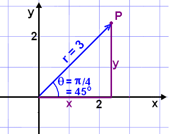
We
use the trig rules in a right angled triangle
cos
![]() = adjacent side/hypotenuse and
= adjacent side/hypotenuse and
sin
![]() = opposite side/hypotenuse.
= opposite side/hypotenuse.
cos
![]() = x/3
= x/3
x = 3 cos 45º ≈ 2.12
sin
![]() =
y/3
=
y/3
y = 3 sin 45º ≈ 2.12
The point P has x-y coordinates (2.12, 2.12).
|
We change polar coordinates to x-y coordinates by using the rules
x = r cos
|
We can draw polar graphs by putting restrictions on either r or
![]() .
For example if we keep
.
For example if we keep
![]() at a constant value and let r take any value we get a straight line graph going
through the origin. If on the other hand we keep r at a constant value and let
at a constant value and let r take any value we get a straight line graph going
through the origin. If on the other hand we keep r at a constant value and let
![]() take all values on the interval
<
take all values on the interval
<
![]() <
2
<
2![]() we get the graph of a circle with centre at the origin and radius the same as
the constant r value.
we get the graph of a circle with centre at the origin and radius the same as
the constant r value.
Polar equations are usually of the form r = f(![]() ).
).
If we want to change an equation given in polar form to an ordinary x-y equation we often have to use quite complicated algebra. Some examples of this are shown in the following.
|
To change from polar equations to x-y equations we use the rules |
Find an x-y equation for the following polar equation:
r = 4/(cos
![]() – sin
– sin
![]() )
)
We begin by multiplying through by (cos
![]() - sin
- sin
![]() )
and then using the rules x = r cos
)
and then using the rules x = r cos
![]() and y = r sin
and y = r sin
![]() .
.
r (cos
![]() – sin
– sin
![]() ) = 4
) = 4
r cos
![]() – r sin
– r sin
![]() = 4
= 4
x – y = 4
y = x – 4
The polar equation r = 4/(cos
![]() – sin
– sin
![]() )
corresponds to the x-y equation y = x – 4.
)
corresponds to the x-y equation y = x – 4.
Find the x-y equation corresponding to the polar equation
r = 2(cos
![]() + sin
+ sin
![]() + 1/r)
+ 1/r)
First multiply both sides of the equation by r and then use the rules
connecting r,
![]() ,
x and y:
,
x and y:
r2
= 2(r cos
![]() + r sin
+ r sin
![]() + 1)
+ 1)
x2 + y2 = 2(x + y + 1)
x2 + y2 = 2x + 2y + 2
Rearranging this we get the familiar equation
x2 – 2x + y2 – 2y = 2
If we add 2 to both sides of the equation we get.
x2 – 2x + 1 + y2 – 2y + 1 = 2 + 2
(x – 1)2 + (y – 1)2 = 22
Which is the equation of a circle with centre (1, 1) and radius 2.
Given the polar equation r = 5 sin 3![]() .
.
We can try to change this to an x–y equation but it does not look promising.
First we‘ll try rewriting
sin 3![]() .
.
sin 3![]() = sin (2
= sin (2![]() +
+
![]() )
)
Now we‘ll use the addition formulas and the formulas for double angles or
simply look up the formula for sin 3![]() .
.
sin 3![]() = 3 sin
= 3 sin
![]() - 4 sin3
- 4 sin3
![]()
Putting this into the given equation gives us
r = 15 sin
![]() - 20 sin3
- 20 sin3
![]()
Multiply through by r3 and using y = r sin
![]() gives us
gives us
r4
= 15 r2·r
sin ![]() - 20
r3 sin3
- 20
r3 sin3
![]()
= 15 r2 y - 20 y3
Now we can use the rule r2 = x2 + y2 and put x2 + y2 in for r2.
r4 = 15 r2 y - 20 y3
(x2 + y2)2 = 15 (x2 + y2)y - 20 y3
x4 + 2x2y2 + y4 = 15x2y + 15y3 - 20 y3
The x-y equation we have found is much more complicated than the original polar equation. This means we need to use the polar equation to draw the graph. We make a table of values.
|
|
r = 5 sin 3 |
|
r = 5 sin 3 |
|
|
0 |
0.0 |
|
0.0 |
|
|
|
3.5 |
13 |
-3.5 |
|
|
|
5.0 |
7 |
-5.0 |
|
|
|
3.5 |
5 |
-3.5 |
|
|
|
0.0 |
4 |
0.0 |
|
|
5 |
-3.5 |
17 |
3.5 |
|
|
|
-5.0 |
3 |
5.0 |
|
|
7 |
-3.5 |
19 |
3.5 |
|
|
2 |
0.0 |
5 |
0.0 |
|
|
3 |
3.5 |
7 |
-3.5 |
|
|
5 |
5.0 |
11 |
-5.0 |
|
|
11 |
3.5 |
23 |
-3.5 |
|
If we make a coordinate system that looks a bit like a spiders web we can easily mark in the points we have found and sketch a graph. We mark one point for each angle and use the value of r to find its distance from the origin.
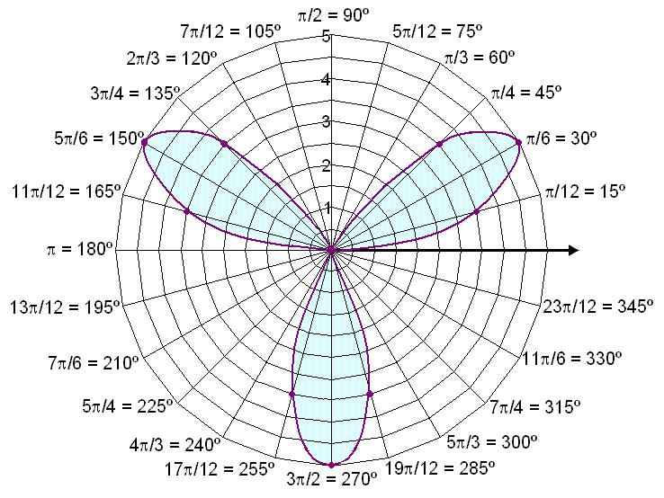
The graph reminds us of a three leaved clover.

Drawing a graph in this way takes a lot of hard work so it‘s very useful to know
how to use the calculator to help.
We choose graph and then use SHIFT and SET UP to make sure the angle is given
in radians.
Next choose V-Window using
.
This gives us the familiar menu window:

We leave this unchanged and scroll down to the next window.
 |
 |
Put in the values shown, pressing
![]() between each step. Minimum (min) 0 and maximum (max) 6.283185 3 which is
approximately 2
between each step. Minimum (min) 0 and maximum (max) 6.283185 3 which is
approximately 2![]() .
In this way we go a complete circle with intervals (pitch) of 2
.
In this way we go a complete circle with intervals (pitch) of 2![]() /100.
/100.
Choosing
![]() takes us back to the graph window.
takes us back to the graph window.

Press F3 (TYPE) to choose the correct type of graph.
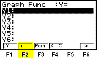
This time we press F2 to choose r =. The graph window shown below opens and we can write in the given equation. (See the shaded line).
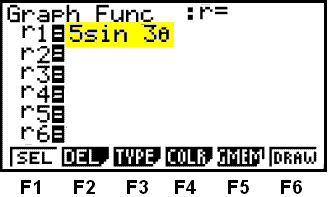
Again we use the
![]() to put
to put
![]() into the equation.
into the equation.
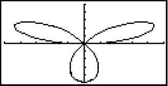
The graph is shown below:
Try Quiz
6
on Vectors.
Remember to use the checklist to keep track of your work.